As everybody knows, statistics is fun. Is there anything cooler than crushing a heap of seemingly uninteresting numbers into gleaming jewels of meaning? Of course not! Models, data-visualization plots, and fat data sets are way cool. So, let’s find an excuse to play with them.
Here’s an excuse
I mean, an important and highly relevant question that many of us share: How many people actually read our blogs? To answer the question, we will need to use statistics, data, and cool plots. Further, if you’ve got the raw data for your blog, you can follow along with your own analysis. Even more fun!
We’ll start with a simple inspection of common web-log data, using command-line tools. After developing a rough understanding of what useful information we can extract, we’ll analyze the raw data using a series of successively more sophisticated techniques. In the end, we will derive a simple formula for estimating readership from easily obtainable data.
Sound good? Then let’s get rocking.
But first, a preemptive strike on would-be poo-pooers: I know all about FeedBurner. I know they will track my blog’s subscribers and use their mystical powers to infer the number of “real” subscribers I have. I know it’s all so easy. But easy isn’t the point. I want to understand what’s going on. Just taking somebody’s word for it isn’t nearly as satisfying as figuring it out yourself – nor as fun.
OK. For real this time, let’s get rocking.
The goal
We want to know how many people read my blog regularly. By regularly, I mean that if I post something today, we want to count the people who will read it within a week’s time. That way we’ll count the weekend readers but not the one-time readers who will trickle in from search engines over the months ahead.
We can’t just look at my web-log stats to determine my blog’s readership, however. That’s because a lot of people read my blog through online feed aggregators, such as Bloglines and Google Reader, and never actually “hit” my blog when they read it. (My blog is so ugly, in fact, that I would expect lots of my readers to use a feed aggregator just to protect themselves from my design “skills.”)
So the goal is to figure out how to count my readers using the data we can actually get our hands on.
The data
Here’s what we have: my HTTP server’s log. That’s it. Can we squeeze the good stuff from it? Let’s find out.
Each entry in the log represents a single request for something on my site. A typical entry looks like this (split over multiple lines for your reading pleasure):
72.14.199.81 - - [19/Aug/2007:19:31:43 -0400]
"GET /xml/atom/article/472/feed.xml HTTP/1.1" 200 1959 "-"
"Feedfetcher-Google; (+http://www.google.com/...; 1 subscribers; ...)"
There’s a lot of potentially useful information in there:
- the IP address of the host that made the request
- the date and time that the request was received
- a summary of the request (e.g., “GET /xml/atom/article/472/feed.xml HTTP/1.1”)
- the response code, typically 200 for a successful response
- the string sent by the requester’s user agent to identify itself (e.g., “Feedfetcher-Google; (*http://www.google.com/feedfetcher.html; 1 subscribers; …)“)
Note that this particular request was made by Google’s Feedfetcher for an Atom feed. Also note that Feedfetcher told us, via its user-agent identification string, how many of its users have subscribed to this particular feed. That’s good stuff we can use.
My blog’s main Atom feed is at /xml/atom/feed.xml. There are other “main” feeds as well , but let’s focus on this one for now. Let’s see who’s been asking for it recently. First, I’ll create a bash-shell function to grab the subset of the log corresponding to 19 August:
$ get_subset() {
    fgrep "GET /xml/atom10/feed.xml" blog_log |
    fgrep 19/Aug/2007;
  }
Then I’ll summarize the user-agent part of that subset’s log entries:
$ get_subset |
  perl -lne 'print $1 if /"([^";(]+)[^"]*"$/' |
  sort | uniq -c | sort -rn
78 NewsGatorOnline/2.0
47 Vienna/2.1.3.2111
38 Mozilla/5.0
27 YandexBlog/0.99.101
21 NewsFire/69
20 Planet Haskell +http://planet.haskell.org/ ...
19 Feedfetcher-Google
19 AppleSyndication/54
14 Zhuaxia.com 1 Subscribers
14 NetNewsWire/2.1b33
13 RssFwd
13 Bloglines/3.1
11 livedoor FeedFetcher/0.01
10 Feeds2.0
8 RssBandit/1.5.0.10
8 Akregator/1.2.6
7 Eldono
6 Netvibes
4 NetNewsWire/3.0
2 trawlr.com
2 Opera/9.21
2 NetNewsWire/3.1b5
2 NetNewsWire/2.1
2 Mozilla/3.0
1 Vienna/2.2.0.2206
1 Vienna/2.1.0.2107
1 NetNewsWire/2.1.1
1 Liferea/1.2.10
1 JetBrains Omea Reader 2.2
1 FeedTools/0.2.26 +http://www.sporkmonger.com/projects/feedtools/
1 Feedshow/2.0Of the user agents that fetched my feed, only some, such as Bloglines and Google Reader, aggregate on behalf of other users, and only some of those mass aggregators reported how many people have subscribed through them:
$ get_subset |
  perl -lne 'print $1 if /"([^"]*?\d+ subscribers?)/i' |
  sort | uniq -c | sort -rn
78 NewsGatorOnline/2.0 (... 22 subscribers
19 Feedfetcher-Google; (... 102 subscribers
14 Zhuaxia.com 1 Subscribers
13 RssFwd (... 1 subscribers
13 Bloglines/3.1 (http://www.bloglines.com; 82 subscribers
11 livedoor FeedFetcher/0.01 (... 1 subscriber
10 Mozilla/5.0 (Rojo 1.0; ... 4 subscriber
7 Eldono (http://www.eldono.de; 1 subscribers
6 Netvibes (http://www.netvibes.com/; 12 subscribers
2 trawlr.com (+http://www.trawlr.com; 4 subscribers
1 Feedshow/2.0 (http://www.feedshow.com; 1 subscriberOf the user agents that don’t report subscriber counts, most are single-user feed readers. The 47 requests from the Vienna-2.1.3.2111 reader, for example, came from 5 distinct IP addresses :
$ get_subset |
  perl -lane 'print $F[0] if m{"Vienna/2.1.3.2111}' |
  sort | uniq -c | sort -rn
22 121.44.xxx.xxx
20 208.120.xxx.xxx
3 69.154.xxx.xxx
1 84.163.xxx.xxx
1 202.89.xxx.xxxDoes that mean I have only 5 distinct readers using Vienna 2.1.3.2111? Not necessarily. The first IP address, for example, could represent a firewall that serves several people from a single corporate campus. So there could, indeed, be more than 5 users lurking behind those addresses, but it’s hard to know for sure.
Thus we can’t rely on feed-fetching statistics to reliably determine the count of readers. The mass aggregators don’t all report their subscriber counts, and the stand-alone aggregators’ fetching habits are not readily interpreted. And, even if we could obtain reliable fetching inferences, that only tells us how many people fetched my blog’s feeds. We want to know how many people read my blog – actually look at the articles.
To do that, we’ll need a more-sophisticated approach.
A different approach: counting image downloads
Every once in a while, I’ll post an article that contains photos or graphs of something I’m trying to explain. Since images like that are included by reference, they are not actually part of the article itself. So when a feed fetcher grabs a syndicated copy of the article, it won’t bother to fetch the images. There’s no need to use the bandwidth unless the person on the other side of the feed actually reads the article, at which time the person’s feed reader can download the images on demand.
Thus we can use the number of image downloads as an estimate of the number of people who actually read my blog. For each article that has images, we can count how many times each image was downloaded during the article’s first week online and take the average of the counts as an estimate of the number of people who read the article.
The image-counting technique isn’t foolproof, however. Requests from people behind proxy servers may never actually make it to my server to be counted, leading to under-counting. Also, some web crawlers fetch images, which may artificially inflate the count of “readers.” Examining the logs, I didn’t see many image requests from crawlers, so our primary concern is under-counting. Since I’m OK with a conservative count, under-counting is acceptable.
Let’s give image-counting a try. On 15 July 2007, I posted a story about a nasty hailstorm that hit my neighborhood. The story included some photos of the storm and its aftermath. Let’s count how many times the second photo in the story was requested on the day the story was posted:
$ fgrep "webcam-2007-07-13--153421.jpg" mc_log |
fgrep 15/Jul/2007 | wc -l884884 times. Many of those downloads, however, were made by just a few requesting hosts. Here are the top ten downloaders:
$ fgrep "webcam-2007-07-13--153421.jpg" mc_log |
  fgrep 15/Jul/2007 |
  perl -lane 'print $F[0]' |
  sort | uniq -c | head
42 84.45.xxx.xxx
27 192.168.xxx.xxx
10 75.182.xxx.xxx
7 83.132.xxx.xxx
7 213.203.xxx.xxx
6 72.173.xxx.xxx
6 67.180.xxx.xxx
6 65.214.xxx.xxx
5 89.98.xxx.xxx
5 85.104.xxx.xxxHow do we interpret these duplicate requests? One way would be to say that each request, duplicate or not, represents a unique reader. It’s plausible. When many readers share a gateway firewall, say in a corporate setting, they will all end up making requests from the same IP address. Thus, if we want to count all such readers, we should count all of the requests.
The more conservative interpretation is that all of the requests from the same IP address represent only a single reader. All of the duplicate requests might be reloads or, perhaps, the work of an overzealous user-agent working on behalf of that user. Let’s recount using this conservative assumption:
$ fgrep "webcam-2007-07-13--153421.jpg" mc_log |
  fgrep 15/Jul/2007 |
perl -lane 'print $F[0]' | sort -u | wc -l635So what’s the real count, 635 or 884? The truth probably lies somewhere in between. To make sure we capture the truth, then, let’s use both interpretations in our ongoing analysis. We will develop low and high estimates from now on.
If you have sharp eyes, you may have noticed that the second IP address in the list above was from a private network. That address, in fact, belongs to my workstation. When I write articles, I frequently reload the drafts, and reloading causes the images within the drafts to be re-fetched. We’ll need to filter out my addresses during our later analyses.
There’s one more thing to consider. We still need to count the image downloads for the rest of the week. So far, we have only counted those for the article’s first day online. So, let’s re-do our conservative count, only this time for the whole week. Let’s also filter out my private addresses and ignore all but HTTP 200 “OK” responses:
$ fgrep "webcam-2007-07-13--153421.jpg" mc_log |
  fgrep " 200 " |  # only count full downloads (status code = 200)
  grep -P '(1[56789]|2[01])/Jul/2007' |  # Jul 15 thru 21 (7 days)
  perl -lane 'print $F[0] unless $F[0] =~ /^192\.168\./' |
sort -u | wc -l1601So, we estimate conservatively that my article on the hailstorm was read by about 1600 people in its first week. Since the article was published on 15 July 2007, we can conservatively estimate that my blog’s regular readership was about 1600 at that time, too.
But that’s just a single point estimate. We’ll need more data if we’re to draw reliable conclusions.
Compiling the image data
To compile enough data for meaningful inferences, I have whipped up a small script to extract and summarize image-download statistics, given an HTTP-server log. Running the script on my blog’s log, here’s what we get:
| Date | Hits low | Hits high | Image |
|---|---|---|---|
| 2006-06-18 | 158 | 192 | lady-beetle-larva-upside-down-small.jpg |
| 2006-06-18 | 157 | 191 | lady-battle-larva-upside-down-close.jpg |
| 2006-07-06 | 163 | 200 | lectro-shirt-before-and-after-wash-small |
| 2006-07-06 | 163 | 203 | lectro-shirt-before-wash-300dpi.jpg |
| 2006-07-06 | 168 | 206 | lectro-shirt-before-wash-small.jpg |
| 2006-07-07 | 155 | 194 | Cladonia-cristatella-close.jpg |
| 2006-07-07 | 155 | 194 | Cladonia-cristatella.jpg |
| 2006-08-03 | 147 | 188 | annies-mixup-0003.jpg |
| 2006-08-03 | 146 | 188 | annies-mixup-0002.jpg |
| 2006-08-24 | 173 | 217 | blog-fd-usage-vs-time.png |
| 2006-09-12 | 271 | 328 | perl-at-work-sign.png |
| 2006-10-18 | 1448 | 1582 | safe-strings.png * |
| 2006-11-04 | 1005 | 1351 | old-web-site-3.png |
| 2006-11-04 | 1011 | 1364 | old-web-site.png |
| 2006-11-14 | 1265 | 1747 | toms-apple-pie.jpg |
| 2007-05-25 | 1567 | 2406 | problem-close.jpg |
| 2007-05-25 | 1563 | 2400 | receiver-insides.jpg |
| 2007-05-25 | 1551 | 2383 | repair.jpg |
| 2007-06-21 | 2290 | 3024 | perl-and-r.png * |
| 2007-07-15 | 1574 | 2360 | webcam-2007-07-13–153751.jpg |
| 2007-07-15 | 1562 | 2379 | backyard-ice.jpg |
| 2007-07-15 | 1553 | 2364 | shredded.jpg |
| 2007-07-15 | 1567 | 2346 | webcam-2007-07-13–153757.jpg |
| 2007-07-15 | 1561 | 2355 | webcam-2007-07-13–153808.jpg |
| 2007-07-15 | 1612 | 2469 | hailstorm2.jpg |
| 2007-07-15 | 1592 | 2382 | webcam-2007-07-13–153726.jpg |
| 2007-07-15 | 1586 | 2381 | webcam-2007-07-13–153747.jpg |
| 2007-07-15 | 1601 | 2404 | webcam-2007-07-13–153421.jpg |
Like most data sets, this one looks better in graphical form:
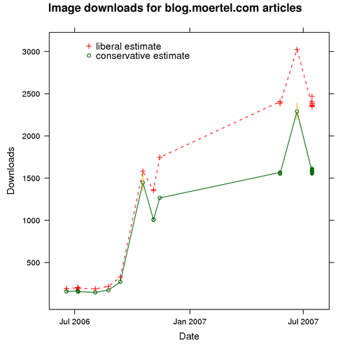
The circles represent our conservative readership estimates, and the pluses represent our liberal readership estimates. To interpret the overall readership trend, focus on one set of estimates, either circles or pluses.
What do we see? First, it looks like the quantity of downloads has increased steadily, from a few hundred in July 2006 to the low thousands by July 2007. That’s nice.
Second, the data are sparse. I don’t post images often, so we don’t have much data to go on.
Third, it looks like we have some outliers. If you look at the points near October 2006 and June 2007, you’ll see that they jump up from the surrounding points. If these jumps truly represented a sudden increase in readership, we would expect them to be permanent, reflected in later readership data. What we see, however, is that these gains are only temporary.
Thus it seems reasonable to conclude that something else is going on for these images. If you look back at the data table, I have marked the pair of curious images with asterisks. As it turns out, both of these images were part of stories that were featured on Reddit. So, what these data reflect is the normal readership plus the Reddit effect. To avoid throwing off our inferences, let’s discard the data for these two images.
In the end, we have a pretty good means of estimating my blog’s readership on the dates when I posted articles that contained images. The problem is, I would like to know what my readership is all the time, not just on those rare occasions I post images. I certainly don’t want to resort to using web bugs. Hey, I’m no marketing weasel.
It’s time to add yet another layer of sophistication to our analysis.
A combined model: reported subscribers with image downloads
Let’s go back to the subscriber numbers reported by online aggregators such as Bloglines and Google Reader. If we assume that those aggregators represent a decent slice of my readers, and that the size of that slice as a proportion of the whole universe of readers doesn’t change much over time, we can model actual readership in terms of reported subscriber numbers. Then, we can use that model to predict actual readership for the dates when no image-download data are available.
That’s the plan. So, let’s get going.
Gathering subscriber data
So, let’s grab those subscriber numbers. Again, I’ve whipped up a Perl script to gather the data. Here’s what the script does. It –
- scans my blog’s HTTP server log
- ignores requests from private networks
- ignores requests that don’t report a subscriber count
- emits one subscriber count for each day of data in the log, computed as the sum of each feed’s subscriber count, as reported by each aggregator
Running the script on my server log, I got a large data set. It’s so large that I’ll go straight to the plot:
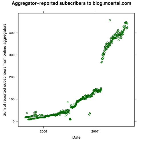
As you would expect, these subscriber counts are less than the corresponding reader counts we gathered from image downloads. Not everybody uses an online feed reader, after all.
One thing that leaps out is the discontinuity around February 2007. What happened back then? As it turns out, that is when Google finally started reporting its subscriber counts. Since Google has a large share of the online aggregator market, that one little change resulted in a big increase in the total of reported counts.
Still, that jump is going to make our analysis a bit more difficult. When we relate subscriber counts to actual readers, we will need to account for the “Google effect.”
Likewise, there are a few other sets of outliers – points that look like bogus data – we should keep in mind. To see whether any of our image-download data coincide with these outliers, let’s highlight our subscriber data for the days when we also have image data:
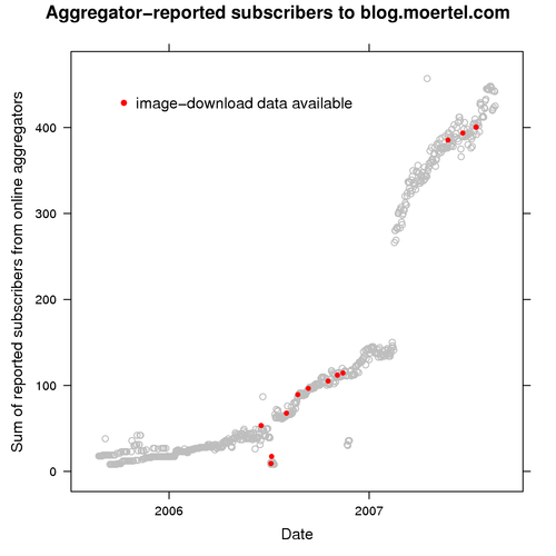
Sure enough, some of our early download data coincide with an outlier group in July 2006. Let’s remove that download data from our analysis set, too.
Our data cleaned, let’s move on.
The model
Now we are ready to relate subscribers to readers . Here’s our model:
yi = a · gi · xi + ei
Where:
- y represents actual readers (as estimated from image downloads)
- x represents subscribers as reported by online aggregators
- i ranges over 1–N for our N data points
- a is the coefficient that relates readers to subscribers
- g is a true/false factor to indicate whether x includes Google Reader users
- e is the model’s error term
What the model says is that readership (y) varies linearly with subscriber counts (x) and that the rate at which it varies is given by a · gi. (Model aficionados may note that this is a varying-slope model.) The model does not include a constant term; this is to fix the y-intercept at 0 because when we have no actual readers, we cannot have any subscribers, either. Thus we know the point (0,0) must be part of the fitted model.
Here’s the data set we will use to fit our model:
  date       y.low y.high   x     g
1 2006-06-18   158    192  53 FALSE
2 2006-08-03   146    188  68 FALSE
3 2006-08-24   173    217  89 FALSE
4 2006-09-12   271    328  97 FALSE
5 2006-11-04  1008   1358 112 FALSE
6 2006-11-14  1265   1747 114 FALSE
7 2007-05-25  1560   2396 385  TRUE
8 2007-07-15  1579   2382 401  TRUE
This data set combines a summarized version of our image-download data set with the corresponding data from our aggregator-reported subscriber set (the red points in the previous plot).
The low and high y values represent our conservative and liberal interpretations of readership, which we discussed earlier. You’ll also note that where multiple images were available for any particular date, I have averaged their download counts to give a centralized readership estimate for that date. (Exercise: For this model, why shouldn’t we include multiple images for a single date?)
Let’s plot this data set (just the y.low part):
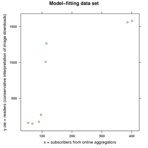
There aren’t many points to go on, but because our model is so simple, there are probably enough. That means it’s time to fit our model to our data.
To fit our linear model, I’ll use the lm function from the amazingly cool R statistics system (which I’ve also been using for our plots). To summarize the results, I’ll use the display function from the arm CRAN package, which accompanies Andrew Gelman and Jennifer Hill’s wonderful book Data Analysis Using Regression and Multilevel/Hierarchical Models. (BTW, Gelman’s blog is fascinating. It’s one of my favorite reads.) If you are following along and don’t have the “arm” package installed, you can use the summary function instead of display.
First, let’s fit the model to the conservative data:
M1.low <- lm (y.low ~ g:x + 0, data=subs.readers)
display(M1.low)
lm(formula = y.low ~ g:x + 0, data = subs.readers)
coef.est coef.se
gFALSE:x 6.31 1.59
gTRUE:x 3.99 0.64
n = 8, k = 2
residual sd = 356.94, R-Squared = 0.90That’s a pretty good fit. Both of our model parameters are significant (even at the 1-percent level). The resulting model says that each subscriber represents about 4 actual readers (or 6.3 readers if the subscriber count doesn’t include Google Reader users).
Let’s visualize the model, now fit to our data:
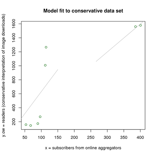
The gray line segments represent our fitted model’s predictions. Thus, for example, when we have x = 100 reported subscribers, the model predicts that we have about y = 630 actual readers. Likewise, when we have 400 subscribers, the model predicts that we have about 1600 actual readers.
The two line segments show how our model accommodates the “Google effect.” On the left, we have the pre-Google slope; on the right, the post-Google slope. In effect, our model combines two simpler models and chooses between them based on the Boolean factor g.
And that’s all there is to the fitting process. Let’s repeat the process for the liberal-interpretation data.
M1.high <- lm (y.high ~ g:x + 0, data=subs.readers)
display(M1.high)
lm(formula = y.high ~ g:x + 0, data = subs.readers)
coef.est coef.se
gFALSE:x 8.46 2.25
gTRUE:x 6.08 0.91
n = 8, k = 2
residual sd = 504.22, R-Squared = 0.91Under this model, each subscriber represents about 6 actual readers (or 8.5 if our subscriber count doesn’t include Google Reader users).
Now that we have our models, let’s use them to predict actual readership.
Using our models for prediction
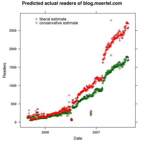
Models ready, we can now predict my blog’s readership for any day, not just those days on which I happened to include images in my postings.
I have subscriber data in an R data frame called, unsurprisingly, subscriber.data. It provides, for each day I have subscriber statistics, values for x and g. (This is the same data set visualized in the earlier plot “Aggregator-reported subscribers to blog.moertel.com.”) We can tell R to plug these values into our model to predict the actual number of readers for those days. Let’s make both conservative and liberal predictions, storing them in a new data frame called predicted.readers:
predicted.readers <-
  transform(subscriber.data,
            readers.low  = predict(M1.low, subscriber.data),
            readers.high = predict(M1.high, subscriber.data))
Now let’s plot our predictions. First the plot code, just so you can see how it’s done in R:
xyplot(readers.low + readers.high ~ date,
       data = predicted.readers,
       main = "Predicted actual readers of blog.moertel.com",
       ylab = "Readers",
       xlab = "Date",
       auto.key = list(x = .35, y = .9, corner = c(0,0),
                       text = c("conservative estimate",
                                "liberal estimate"),
                       reverse.rows = T, between = -19))
And the resulting plot:
The bottom line
We have distilled a ton of raw data into a simple formula for predicting my blog’s actual readership from readily available subscriber counts. Just take the total subscriber count and multiply by 4 and 6, respectively, for low and high estimates of readership.
So, to answer our original question, how many readers does my blog have? Only a few days ago, on 18 August, the online aggregators reported that they were serving my feeds to 442 subscribers. So we can predict that, right now, my blog has 1750 to 2650 readers.
We have our answer. Getting it took some doing, but the doing was fun, so all’s good.
Certainly, we could go on. There are many interesting questions left to be answered. What, for example, is the growth trend of my readership? What is Google Reader’s market share? For now, however, it’s time to take a break.
I hope you had fun following along. If you have your own data, I’d be interested in hearing about your analytical explorations. (And, if you haven’t installed R on your computer yet, do it now. R is seriously cool and comes with great documentation, examples, and sample data. If you’re not using R, you’re not having all the fun you deserve.)
Update: minor editing tweaks for clarity.